Most charts and maps on this site were created with the Stata statistical software package. This guide explains how maps like those with adult and youth literacy rates in 2010 can be created with Stata. The article supersedes an earlier version from 2005 and introduces updated maps with current country borders. For example, South Sudan, which seceded from Sudan in 2011, is shown as a separate country on the new maps. The instructions below are for Stata version 9 or later. Users of Stata 8 are referred to the guide from 2005. The creation of maps is not supported in older versions of Stata.
Requirements
- Stata version 9.2 or later.
- spmap: Stata module for drawing thematic maps, by Maurizio Pisati. spmap can be installed in Stata with this command:
ssc install spmap - shp2dta: Stata module for converting shapefiles to Stata format, by Kevin Crow. shp2dta can be installed in Stata with this command:
ssc install shp2dta - Shapefile: A shapefile is a data format for geographic information systems. For the maps in Figures 1 and 2, please download this public domain shapefile from Natural Earth:
ne_110m_admin_0_countries.zip (184 KB, world map with country borders, scale 1:110,000,000) - Note: The instructions are accurate for Natural Earth maps version 2.0.0, the most recent version of the maps available in April 2014.
Step 1: Convert shapefile to Stata format
- Unzip ne_110m_admin_0_countries.zip to a folder that is visible to Stata, for example the current working directory of Stata. The archive contains six files:
ne_110m_admin_0_countries.dbf
ne_110m_admin_0_countries.prj
ne_110m_admin_0_countries.shp
ne_110m_admin_0_countries.shx
ne_110m_admin_0_countries.README.html
ne_110m_admin_0_countries.VERSION.txt - Start Stata and run this command:
shp2dta using ne_110m_admin_0_countries, data(worlddata) coor(worldcoor) genid(id) - Two new files will be created: worlddata.dta (with the country names and other information) and worldcoor.dta (with the coordinates of the country boundaries).
- If you plan to superimpose labels on a map, for example country names, run the following command instead, which adds centroid coordinates to the file worlddata.dta:
shp2dta using ne_110m_admin_0_countries, data(worlddata) coor(worldcoor) genid(id) genc(c) - Please refer to the spmap documentation to learn more about labels.
- The DBF, PRJ, SHP, and SHX files are no longer needed and can be deleted.
Step 2: Draw map with Stata
- Open worlddata.dta in Stata.
- For the example maps, create a variable with the length of each country's name. The Stata command for this is:
generate length = length(admin) - Draw a map that indicates the length of all country names with this command:
spmap length using worldcoor.dta, id(id) - The default map (Figure 1) is grayscale, it shows Antarctica, there are four classes for the length of the country names, the legend is very small, and the legend values are arranged from high to low.
Figure 1: Length of country names (small scale map, default style)
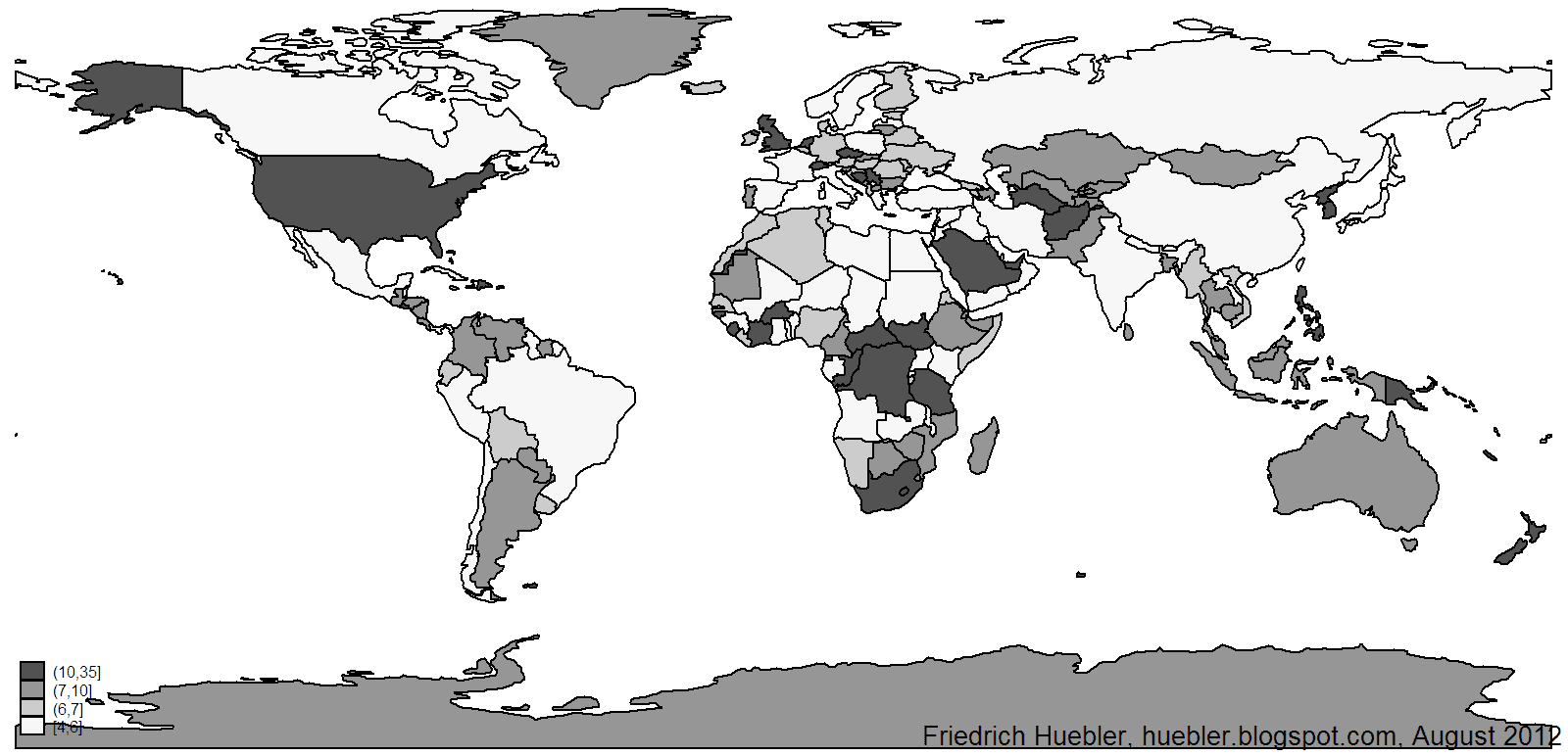
Click image to enlarge.
- A second map without Antarctica, with a blue palette, five classes, and with a bigger legend with values arranged from low to high (Figure 2) can be drawn with this command:
spmap length using worldcoor.dta if admin!="Antarctica", id(id) fcolor(Blues) clnumber(5) legend(symy(*2) symx(*2) size(*2)) legorder(lohi) - Darker colors on the map indicate longer country names, ranging from 4 (for example Cuba and Fiji) to 35 characters (French Southern and Antarctic Lands).
- Please read the Stata help file for spmap to learn about the many additional options for customization of maps.
Figure 2: Length of country names (small scale map, blue palette)
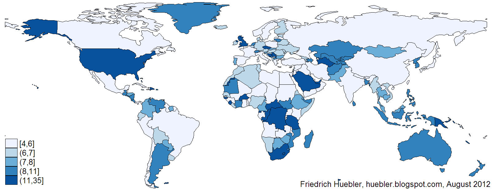
Click image to enlarge.
Alternative maps with more detail
The shapefile that was used for Figures 1 and 2 was designed for small maps. It contains the borders for 177 countries and territories and does not include smaller geographic units like Hong Kong, Monaco, or St. Vincent and the Grenadines. As an alternative to the small scale map in Figures 1 and 2, Natural Earth offers shapefiles with more detail that were designed for larger maps.
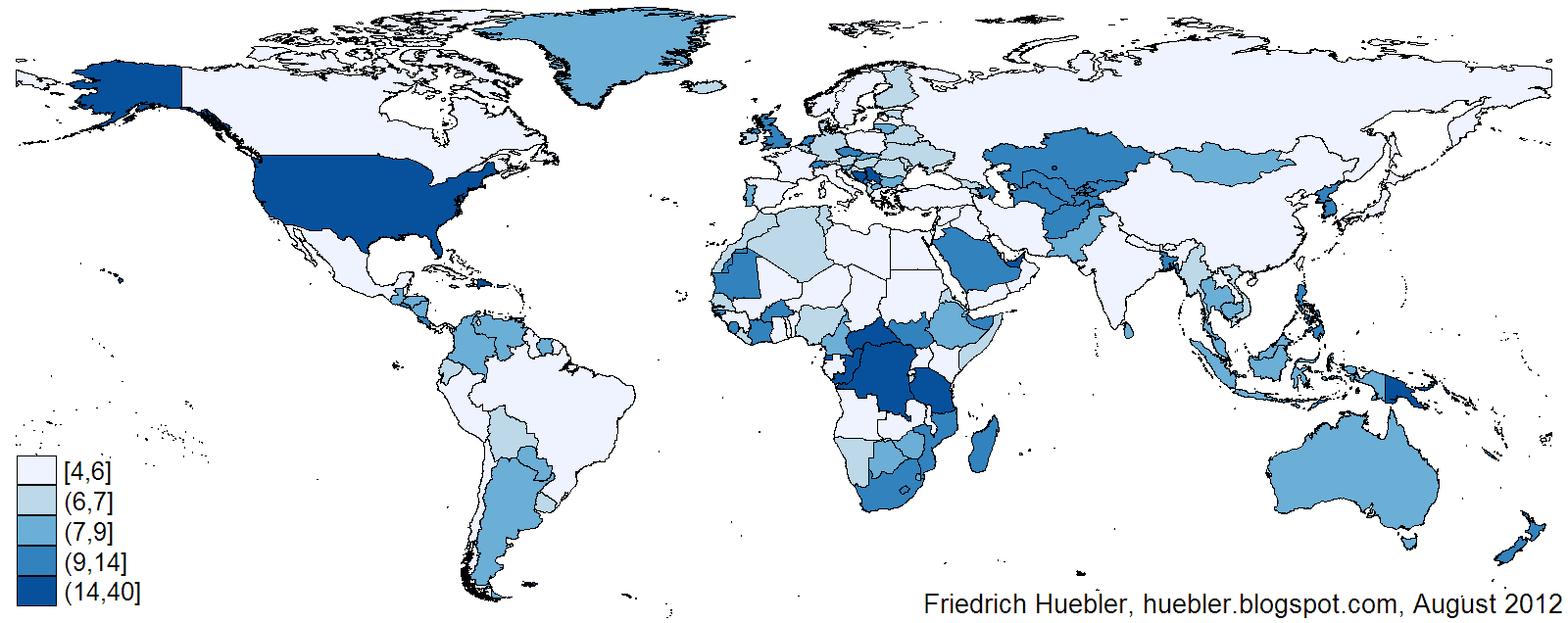
- To create the map in Figure 3, download this shapefile from Natural Earth, which has information for 241 countries and territories:
ne_50m_admin_0_countries.zip (799 KB, world map with country borders, scale 1:50,000,000) - Unzip ne_50m_admin_0_countries.zip to a folder that is visible to Stata.
- Run this Stata command to convert the shapefile to Stata format:
shp2dta using ne_50m_admin_0_countries, data(worlddata2) coor(worldcoor2) genid(id) - If you need Stata files with centroids, run this command instead:
shp2dta using ne_50m_admin_0_countries, data(worlddata2) coor(worldcoor2) genid(id) genc(c) - Open worlddata2.dta in Stata.
- Create a variable with the length of each country's name:
generate length = length(admin) - Draw the map in Figure 3:
spmap length using worldcoor2.dta if admin!="Antarctica", id(id) fcolor(Blues) clnumber(5) legend(symy(*2) symx(*2) size(*2)) legorder(lohi) - The map takes longer to draw than the map in Figures 1 and 2 because it is more detailed and shows more geographic units. The names of the countries and territories on the map have a length up to 40 characters (South Georgia and South Sandwich Islands).
Figure 3: Length of country names (medium scale map)

Click image to enlarge.
- To create the map in Figure 4, download this shapefile from Natural Earth, which has information for 255 countries and territories, including small islands like the Ashmore and Cartier Islands:
ne_10m_admin_0_countries.zip (5.1 MB, world map with country borders, scale 1:10,000,000) - Unzip ne_10m_admin_0_countries.zip to a folder that is visible to Stata.
- Run this Stata command to convert the shapefile to Stata format:
shp2dta using ne_10m_admin_0_countries, data(worlddata3) coor(worldcoor3) genid(id) - If you need Stata files with centroids, run this command instead:
shp2dta using ne_10m_admin_0_countries, data(worlddata3) coor(worldcoor3) genid(id) genc(c) - Open worlddata3.dta in Stata.
- Create a variable with the length of each country's name:
generate length = length(ADMIN) - Draw the map in Figure 4:
spmap length using worldcoor3.dta if ADMIN!="Antarctica", id(id) fcolor(Blues) clnumber(5) legend(symy(*2) symx(*2) size(*2)) legorder(lohi) - The map takes longer to draw than the maps in Figures 1, 2 and 3 because it has the largest amount of detail. The differences between the maps in Figures 3 and 4 can be seen by clicking on the images to enlarge them. Figure 4 has more islands and more detailed shorelines. The names of the countries and territories on the map in Figure 4 have a length up to 40 characters (South Georgia and South Sandwich Islands).
Figure 4: Length of country names (large scale map)
Click image to enlarge.
Software used in this guide
- Stata: statistical software package
- spmap: Stata module for drawing thematic maps, by Maurizio Pisati
- shp2dta: Stata module for converting shapefiles to Stata format, by Kevin Crow
- ne_110m_admin_0_countries.zip: small scale (1:110,000,000) Natural Earth world map with country borders (184 KB)
- ne_50m_admin_0_countries.zip: medium scale (1:50,000,000) Natural Earth world map with country borders (799 KB)
- ne_10m_admin_0_countries.zip: large scale (1:10,000,000) Natural Earth world map with country borders (5.1 MB)
Related articles
- Adult and youth literacy in 2010
- Guide to creating maps with Stata (previous version of this guide, from 2005)
- Guide to integrating Stata and external text editors
External links
- Natural Earth maps (public domain shapefiles)
- Stata FAQ: How do I graph data onto a map with spmap?
- Shapefile (Wikipedia)
- Geographic information system (Wikipedia)
- Centroid (Wikipedia)
Permanent URL: http://huebler.blogspot.com/2012/08/stata-maps.html

